Introduction

Most data engineering tutorials hand you a clean CSV file and say, "Here, load this into a table." Real life is nothing like that.

In the real world, your data source is an HTTP API that sometimes returns malformed timestamps. The field your downstream team depends on shows up as null three percent of the time. Someone submits the same order twice. The infrastructure your pipeline runs on needs to be reproducible so your colleague can set it up on their own machine without a four-hour phone call.

That is the gap this article fills.

We will build a pipeline that handles all of those problems, on real cloud infrastructure, with real code. Here is what we are building:

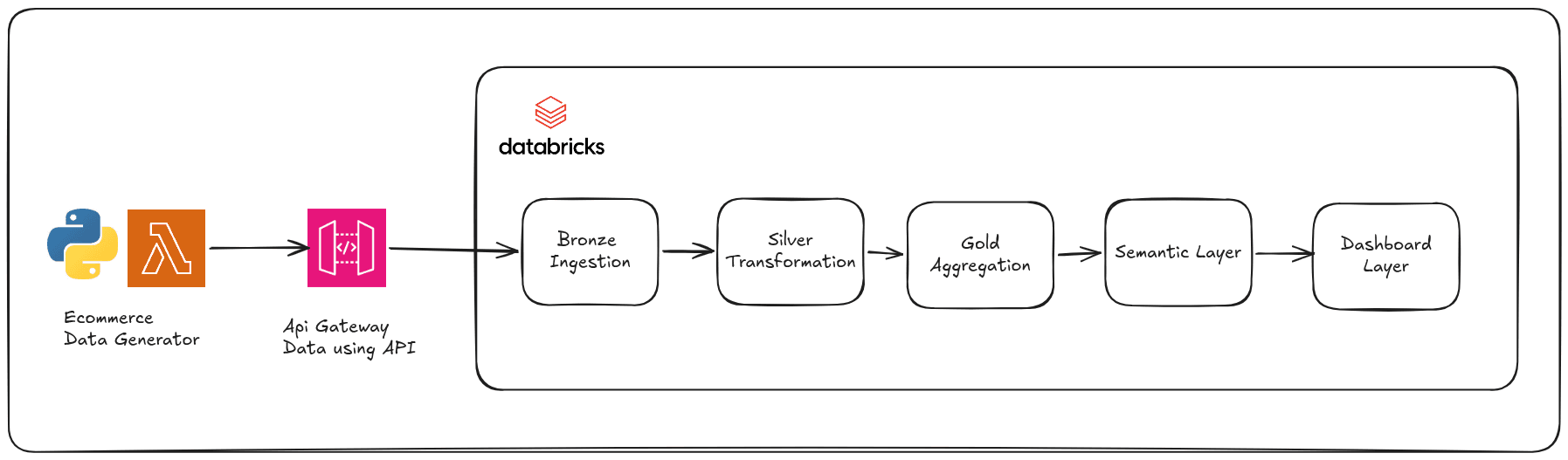
A synthetic e-commerce data generator deployed on AWS Lambda, exposed via AWS API Gateway, provisioned entirely with Terraform
A three-layer Medallion pipeline (Bronze, Silver, Gold) in Databricks, built on Delta Lake
A Star Schema dimensional model with a semantic layer of SQL views
A Seaborn-powered analytics dashboard reading directly from those views

The data source is a live HTTP API we control. Every call returns a fresh batch of e-commerce transactions, and about 8 percent of them contain intentional quality problems: malformed dates, missing prices, duplicate order IDs. Our pipeline has to handle all of it.

What you need to follow along:

Basic Python (you can read a for-loop and a dict)
Basic SQL (you know what SELECT and GROUP BY do)
An AWS account (free tier is fine)
A Databricks Community Edition account (completely free)

No prior AWS, Terraform, or Databricks experience required.

Let's Proceed with Implementation

1. The Data Generator: Simulating a Real Source System

Before we touch any infrastructure, let us talk about what data we are generating and why the design choices matter.

Why Build a Generator Instead of Using a Public Dataset?

Public datasets are static. You download a file, it never changes, and you cannot inject the specific edge cases your pipeline needs to handle. Building our own generator gives us two things a static file cannot: a live HTTP API that simulates a real source system, and precisely controlled dirty data so we know exactly what our pipeline should catch.

What a Transaction Record Looks Like

Every call to our API produces e-commerce transaction records that look like this:

{
  "order_id": "a3f8c2b1-...",
  "customer_id": 4821,
  "customer_name": "Sarah Connor",
  "email": "sarah.connor@email.com",
  "product": "Wireless Headphones",
  "category": "Electronics",
  "quantity": 2,
  "price": 149.99,
  "region": "US-East",
  "timestamp": "2026-04-18T14:32:01",
  "status": "completed"
}

The catalog contains 15 products across 5 categories: Electronics, Accessories, Clothing, Fitness, and Home. Customers come from 5 regions: US-East, US-West, EU-West, EU-Central, and APAC.

The Intentional Dirty Data

This is the part that makes the pipeline realistic. Three types of quality problems are injected at specific rates:

Malformed timestamps (5% of records): The timestamp field is replaced with values like "not-a-date", "2026/13/45", "yesterday", or "". These will fail any timestamp parsing and need to be quarantined.

Missing fields (3% of records): Either quantity or price is deleted from the record entirely. In the downstream pipeline, a missing price means the order's revenue cannot be calculated, so it gets quarantined. A missing quantity gets defaulted to 1 (a documented business assumption).

Duplicate order IDs (2% of records): A record is assigned an order ID that already appeared earlier in the same batch. This simulates client-side retry logic, which is extremely common in real API integrations.

Here is the core of the generator function:

def generate_transaction(existing_order_ids=None):
    product = random.choice(PRODUCTS)
    record = {
        "order_id":       str(uuid.uuid4()),
        "customer_id":    random.randint(1000, 9999),
        "customer_name":  fake.name(),
        "email":          fake.email(),
        "product":        product,
        "category":       PRODUCT_CATALOG[product],
        "quantity":       random.randint(1, 10),
        "price":          round(random.uniform(5.99, 999.99), 2),
        "region":         random.choice(REGIONS),
        "timestamp":      _random_timestamp(),
        "status":         random.choice(STATUSES),
    }
    if random.random() < 0.05:
        record["timestamp"] = random.choice(MALFORMED_TIMESTAMPS)
    if random.random() < 0.03:
        del record[random.choice(["quantity", "price"])]
    if existing_order_ids and random.random() < 0.02:
        record["order_id"] = random.choice(existing_order_ids)
    return record

Notice that customer_name and email are generated by the Faker library. These are PII fields. One of the things the Silver layer will do is hash the emails and mask the names before the data reaches any analytics table.

The Lambda entry point accepts a count query parameter (defaulting to 100, capped at 5000) and returns all the generated records as a JSON array:

def lambda_handler(event, context):
    params = event.get("queryStringParameters") or {}
    count  = int(params.get("count", 100))
    count  = max(1, min(count, 5000))

    transactions = []
    order_ids    = []
    for _ in range(count):
        txn = generate_transaction(existing_order_ids=order_ids)
        transactions.append(txn)
        order_ids.append(txn["order_id"])

    return {
        "statusCode": 200,
        "headers": {"Content-Type": "application/json"},
        "body": json.dumps(transactions),
    }

2. AWS Services: What Each One Does in This Project

Three AWS services make this work. Let us go through each one concretely.

AWS Lambda: The Serverless Function Runtime

Think of Lambda as a function in the cloud that runs only when called. You upload your Python code, AWS handles the server, the OS, the scaling, and the networking. You pay only for the milliseconds your code actually runs. For a data generator that is called a few times a day, this costs essentially nothing.

In this project, the Lambda function is the data generator. When your Databricks notebook wants a fresh batch of transactions, it makes an HTTP GET request. API Gateway receives that request and invokes the Lambda function. Lambda runs lambda_handler()generates the records, and returns them as JSON.

The function is deployed using Python 3.12. It uses the Faker library to generate realistic names and email addresses, which is packaged as a separate Lambda Layer (more on that below).

Lambda Layers: The Faker library is not included in the Lambda function's zip file. Instead, it is packaged as a Lambda Layer, which is a way to share dependencies across multiple functions without bundling them into each deployment package. The layer is uploaded once, and the function references it by ARN.

The build.sh script handles both packaging steps:

# Build the Faker layer
pip install faker -t python/ --quiet --no-cache-dir
zip -r9 faker_layer.zip python/

# Package the handler
zip -j function.zip handler.py

CloudWatch Logs: Every Lambda invocation automatically writes logs to AWS CloudWatch with a 7-day retention period. This keeps costs low while preserving enough history to debug any issues.

AWS IAM: Who Is Allowed to Do What

IAM (Identity and Access Management) is how AWS controls permissions. Every service and user that calls an AWS API needs an IAM identity, and that identity needs explicit permission for every action it takes.

Lambda functions are no exception. To run, our function needs an IAM Role, which is an identity that Lambda can assume when it runs. The role has two things attached to it:

The trust policy: This answers the question "who is allowed to assume this role?" Our trust policy says only the Lambda service (lambda.amazonaws.com) can assume it:

data "aws_iam_policy_document" "lambda_assume_role" {
  statement {
    effect  = "Allow"
    actions = ["sts:AssumeRole"]
    principals {
      type        = "Service"
      identifiers = ["lambda.amazonaws.com"]
    }
  }
}

The execution policy: This answers the question "what is this role allowed to do?" We attach the AWS-managed AWSLambdaBasicExecutionRole policy, which grants exactly one permission: the ability to write logs to CloudWatch. Our generator does not read from S3 or write to DynamoDB or anything else, so this minimal policy is all it needs.

This is the principle of least privilege in action. Grant only the permissions required for the specific task, nothing more.

The PassRole note: If you are setting up the IAM user that runs Terraform, you will need to grant it the iam:PassRole permission explicitly. This is a common gotcha: even if your user has full IAM permissions, AWS requires a specific PassRole grant before you can attach a role to a Lambda function. The Terraform state in this project documents the resource ARN format you need.

AWS API Gateway (HTTP API v2): The Public Door

Lambda functions are not directly callable from the internet by default. API Gateway is the front door that receives HTTP requests and forwards them to Lambda.

We use the HTTP API type (v2), not the older REST API (v1). HTTP APIs are cheaper, simpler, and have lower latency. For a straightforward GET endpoint with no authentication, it is the right choice.

Here is how the request flow works:

A client sends GET https://{api-id}.execute-api.us-east-1.amazonaws.com/transactions?count=200
API Gateway matches the route GET /transactions and triggers the Lambda integration
The integration type is AWS_PROXY, which passes the raw event object (including query string parameters) directly to the Lambda function
Lambda processes the request and returns a response dict
API Gateway forwards that response back to the client

Client Request
     |
     v
API Gateway (Route: GET /transactions)
     |
     v
Lambda Integration (AWS_PROXY, payload format 2.0)
     |
     v
lambda_handler(event, context)
     |
     v
JSON response with transactions

The stage is set to $default with auto_deploy = true, which means every Terraform apply immediately publishes the latest configuration without a manual deployment step.

API Gateway also has its own CloudWatch Log Group for access logs, recording the request ID, source IP, HTTP method, route, status code, and response length for every request.

One final piece: the Lambda permission. API Gateway cannot invoke Lambda unless Lambda explicitly grants it permission. This resource in Terraform creates that grant:

resource "aws_lambda_permission" "api_gw" {
  statement_id  = "AllowAPIGatewayInvoke"
  action        = "lambda:InvokeFunction"
  function_name = aws_lambda_function.data_generator.function_name
  principal     = "apigateway.amazonaws.com"
  source_arn    = "${aws_apigatewayv2_api.ecom_api.execution_arn}/*/*"
}

Terraform: Infrastructure as Code

Why Terraform?

Think about the alternative: you log into the AWS console, click around to create a Lambda function, click around to create an IAM role, attach a policy, create an API Gateway, configure the integration, set up the route... and two weeks later, when something breaks, you have no record of what you clicked. Or worse, you need to recreate it in a different AWS account, and you have to remember every decision you made.

Terraform solves this. Your infrastructure is described in .tf files that live in version control alongside your code. To deploy, you run terraform apply. To tear everything down and recreate it from scratch, you run terraform destroy then terraform apply again. The entire process is repeatable and reviewable.

Project Structure

terraform/
  main.tf          -- Provider config and Terraform version constraints
  variables.tf     -- Input variables (region, project name, Lambda config)
  iam.tf           -- IAM role and execution policy
  lambda.tf        -- Lambda function, Faker layer, CloudWatch log group
  api_gateway.tf   -- HTTP API, integration, route, stage, permissions
  outputs.tf       -- Values printed after deploy (the API endpoint URL)

Splitting infrastructure into separate files by concern makes it much easier to find what you are looking for. Everything related to IAM is in iam.tf. Everything related to Lambda is in lambda.tf. Terraform treats all .tf files in a directory as one combined configuration, so there is no extra wiring needed.

Key Configuration Values

The variables.tf file defines all the tunable parameters:

variable "project_name" {
  default = "aws-databricks-ecom-pipeline"
}

variable "aws_region" {
  default = "us-east-1"
}

variable "lambda_runtime" {
  default = "python3.12"
}

variable "lambda_timeout" {
  default = 30   # seconds
}

variable "lambda_memory" {
  default = 256  # MB
}

All resource names are prefixed with var.project_name , so every resource in AWS is clearly identified as belonging to this project. For example, the Lambda function is named aws-databricks-ecom-pipeline-data-generator, the IAM role is aws-databricks-ecom-pipeline-lambda-role, and so on. Consistent naming is what keeps a multi-service AWS account navigable.

Default tags are applied to every resource through the provider block:

provider "aws" {
  region = var.aws_region
  default_tags {
    tags = {
      Project     = var.project_name
      Environment = "dev"
      ManagedBy   = "terraform"
    }
  }
}

Deploying the Infrastructure

Before running Terraform, you need to package the Lambda code. The build.sh script handles this:

cd lambda && bash build.sh

This creates two zip files:

lambda/function.zip containing handler.py
lambda/faker_layer.zip containing the Faker library in Lambda layer format (python/ subdirectory)

With those files in place, deploying is three commands:

cd terraform
terraform init    # download the AWS provider plugin
terraform plan    # preview what will be created
terraform apply   # create everything

After terraform apply completes successfully, the output section prints the API endpoint:

Outputs:

api_endpoint         = "https://abc123xyz.execute-api.us-east-1.amazonaws.com/transactions"
lambda_function_name = "aws-databricks-ecom-pipeline-data-generator"
api_id               = "abc123xyz"

Smoke Testing the API

Once deployed, you can verify the endpoint works with a simple curl command:

curl "https://abc123xyz.execute-api.us-east-1.amazonaws.com/transactions?count=3"

You should get back a JSON array of three transaction records. Some will have clean data, some may have the injected quality problems.

If you get a 200 response with data, everything is wired up correctly. The Lambda function is running, the IAM role is granting it CloudWatch access, and API Gateway is routing requests to it properly.

3. Medallion Architecture and Data Schema

Why Data Pipelines Need Layers

Here is a question worth thinking about before writing a single line of pipeline code: what happens when your transformation logic has a bug?

Let us say you cleaned the raw data and overwrote the original. You find the bug three days later. The original data is gone. You have to go back to the source and re-fetch everything, hope the source still has it, and re-run the entire process.

Now imagine instead that you always kept the raw data exactly as it arrived, and every transformation wrote to a separate table. The original is always there. Fix the bug, re-run from the raw data, done.

That is the core idea behind the Medallion Architecture.

The Medallion Architecture

The name comes from the three tiers, each represented as a layer:

Raw API Response
      |
      v
  BRONZE LAYER         Raw data, exactly as received
      |                Append-only, immutable
      v
  SILVER LAYER         Cleaned, validated, PII-safe
      |                Deduplicated, typed, business-ready
      v
  GOLD LAYER           Analytics-optimised Star Schema
                       Dimension tables + Fact table

Each layer has a contract. Break the contract, and the architecture stops working correctly.

Bronze: Trust Nothing, Store Everything

The Bronze layer has exactly one rule: store data exactly as it arrived.

No cleaning. No filtering. No transformations. If a record has a malformed timestamp, it goes into Bronze with the malformed timestamp intact. If a field is missing, it goes in with the field missing. Bronze is the immutable record of what your source system produced.

Why? Because your Silver transformation logic may have a bug. Or your understanding of the data quality rules may change. Or a business stakeholder may ask, "What did the data actually look like on April 15th?" With an immutable Bronze layer, you can always answer that question. Without it, you are guessing.

Bronze also uses append semantics. Every pipeline run adds rows. Nothing is ever overwritten. If you run the ingestion notebook five times, Bronze will have five batches of data, each identified by a unique _batch_id.

Silver: Earned Trust

Silver takes Bronze data and applies a documented set of transformations to produce something the rest of the business can trust.

In this project, Silver does five things in order:

Timestamp validation - parse the timestamp string and quarantine records where parsing fails
Null field handling - quarantine records missing price, default missing quantity to 1
Type casting - ensure every column has a stable, predictable data type
Deduplication - for duplicates order_id values, keep the most recently ingested record
PII anonymization - hash email with SHA-256, mask customer_name to an initial

Notice what Silver does not do: it does not change the schema, add new business metrics, or restructure the data into a different shape. That is Gold's job.

Gold: Designed for Questions

Gold takes the clean Silver data and restructures it into a shape optimised for analytics queries. In our case, that shape is a Star Schema.

The Data Schema: A Star Schema

The Silver table is a clean, flat transaction log. One row per order, one column per field. That is great for storage and auditing, but imagine you are a business analyst who wants to answer the question "what was revenue by product category on weekends in Q1?"

With the flat Silver table, you would need to extract the date from the timestamp, calculate whether it was a weekend, filter by quarter, group by category, and sum the revenue. That is five operations in a single query, and every analyst who asks a similar question writes those five operations again.

A Star Schema solves this. You pre-compute the repetitive parts into dimension tables and store the answers to the most common groupings as separate, joinable tables. Business queries become fast two-table joins instead of complex multi-step transformations.

Star Schema vs Snowflake Schema

These two terms come up constantly in data engineering discussions. The difference is in how dimension tables are structured:

Star Schema: Dimension tables are flat. A dim_product table has both the product name and the category in the same row. To get "revenue by category", you join fact_orders to dim_product and group by dp.category. One join.

Snowflake Schema: Dimensions are further normalised. dim_product would contain only the product name and a category_key foreign key. There would be a separate dim_category table. To get "revenue by category", you need fact_orders JOIN dim_product JOIN dim_category. Two joins.

We chose Star Schema because a category is simply an attribute of a product. It does not have its own attributes worth breaking out. The Wireless Headphones product is in the Electronics category, full stop. Adding a separate dim_category table would add query complexity with zero analytical benefit.

The Five Tables in Our Gold Layer

             dim_date
             (date_key INT PK)
                  │
dim_customer ─── fact_orders ─── dim_product
(customer_id)    (revenue,        (product_key INT SK)
                  quantity,
                  price)
                  │
             dim_region
             (region_key INT SK)

dim_date

Calendar attributes for every date that appears in the data.

Column	Type	Example
date_key	INT	20260418
order_date	DATE	2026-04-18
day_of_week_num	INT	6
day_name	STRING	Friday
day_of_month	INT	18
week_of_year	INT	16
month_num	INT	4
month_name	STRING	April
quarter	INT	2
year	INT	2026
is_weekend	BOOLEAN	false

The date_key is formatted as an integer in YYYYMMDD format (e.g. 20260418). This is a standard data warehouse pattern. Integer keys are smaller than string keys, sort correctly without any special handling, and are human-readable at a glance.

The is_weekend flag is pre-computed here so every query that needs weekend analysis is just WHERE is_weekend = TRUE instead of WHERE dayofweek(timestamp) IN (1, 7).

dim_customer

One row per unique customer, containing only PII-safe fields. The customer_id (1000-9999) serves as both the natural key and the primary key. When the same customer appears in multiple batches, we keep only the most recently ingested version using a Window function ranked by _ingested_at. This is the SCD Type 1 (Slowly Changing Dimension) strategy: overwrite with the latest.

Column	Type	Example
customer_id	INT	4821
customer_name	STRING	S***
email	STRING	a3f8...c2b1 (SHA-256 hash)

dim_product

One row per product, with a generated surrogate key.

Column	Type	Example
product_key	INT	1
product	STRING	Wireless Headphones
category	STRING	Electronics

The product_key is generated using ROW_NUMBER() OVER (ORDER BY product). This surrogate key is stable across runs because the product catalog does not change. The fact table stores product_key rather than the product name string, which keeps the fact table compact and makes joining efficient.

dim_region

One row per region, with a generated surrogate key.

Column	Type	Example
region_key	INT	1
region	STRING	US-East

Five regions: US-East, US-West, EU-West, EU-Central, APAC.

fact_orders

The center of the star. One row per transaction, with foreign key references to all four dimensions, plus all the measures.

Column	Type	Description
order_id	STRING	The transaction identifier
customer_id	INT	FK to dim_customer
product_key	INT	FK to dim_product
region_key	INT	FK to dim_region
date_key	INT	FK to dim_date
quantity	INT	Units ordered
price	DOUBLE	Unit price
revenue	DOUBLE	price * quantity, pre-computed
status	STRING	completed / returned / pending
_ingested_at	TIMESTAMP	When this record hit Bronze
_batch_id	STRING	UUID of the ingestion run

A few design decisions worth calling out:

revenue is pre-computed. We calculate ROUND(price * quantity, 2) once when building the fact table, and store it as a column. Every subsequent query that needs revenue just reads fo.revenue instead of computing it again. Calculate once, use many times.

status is a degenerate dimension. It has only three values (completed, returned, pending) and no additional attributes. It does not get its own dim table; it stays in the fact table. This is standard practice for low-cardinality attributes with no extra columns to extract.

_ingested_at and _batch_id flow through from Bronze. These metadata columns are preserved all the way from Bronze to the fact table. If a bug ever appears in the Gold layer, you can trace any fact row back to the exact batch of Bronze records it came from.

The Quarantine Pattern

Before closing out the data schema discussion, let us look at one of the most important quality patterns in this pipeline: the quarantine table.

When the Silver notebook encounters a bad record (malformed timestamp, missing price), it does not silently drop it. It writes it to a separate silver_quarantine Delta table with an additional column: _quarantine_reason.

The quarantine reason can be either malformed_timestamp or missing_price. At the end of every Silver run, a data quality report is printed:

Why does this matter? Because the quarantine table is queryable. If next week the quarantine rate jumps from 8% to 40%, you will know something changed upstream in the Lambda function. The quarantine table is your early warning system.

Silently dropping bad records produces clean tables that are hiding a problem you do not know about. Quarantining bad records produces clean tables where you know exactly what did not make it and why.

Referential Integrity Checks

After building the Gold layer, we validate that every foreign key in fact_orders actually resolves to a row in the corresponding dimension table. This is called a referential integrity check.

dim_product_keys = [r.product_key for r in dim_product.select("product_key").collect()]
dim_region_keys  = [r.region_key  for r in dim_region.select("region_key").collect()]
dim_date_keys    = [r.date_key    for r in dim_date.select("date_key").collect()]

orphan_product = df_fact.filter(~F.col("product_key").isin(dim_product_keys)).count()
orphan_region  = df_fact.filter(~F.col("region_key").isin(dim_region_keys)).count()
orphan_date    = df_fact.filter(~F.col("date_key").isin(dim_date_keys)).count()

If any of these counts are greater than zero, there is a join logic bug. Catching it here, at build time, is far better than discovering it six months later when a dashboard shows mysteriously missing revenue.

Understanding how the Code Works

What is Databricks?

Before diving into code, let us set the context. Databricks is a cloud data platform built on top of Apache Spark. You write Python (PySpark) or SQL in notebooks, and a cluster of machines executes it in parallel. For this project, we use Databricks Community Edition, which is completely free.

Think of it like a Jupyter notebook, but instead of running on your laptop, it runs on a cluster. And instead of pandas working on a single machine's memory, Apache Spark distributes the work across multiple nodes and processes data at any scale.

For our pipeline, the notebooks are organized as a sequence:

00_test_connection.ipynb   -- verify Databricks can reach the AWS API
01_bronze_ingestion.ipynb  -- fetch from API, write raw Bronze table
02_silver_transformation.ipynb -- clean, validate, anonymize
03_gold_aggregation.ipynb  -- build Star Schema (dims + fact)
04_semantic_layer.ipynb    -- create KPI SQL views
05_dashboard.ipynb         -- render Seaborn charts

Each notebook reads from the output of the previous one. Running them in order runs the full pipeline end-to-end.

What is Delta Lake?

Delta Lake is a storage layer that sits on top of Parquet files and adds capabilities that are essential for production data pipelines.

Without Delta Lake, if a Spark job writing to a Parquet table crashes halfway through, you end up with a partially written table in an unknown state. Querying it gives you unpredictable results.

Delta Lake adds four things that fix this:

ACID Transactions: Every write either fully succeeds or fully fails. There is no halfway. If a job crashes mid-write, the table stays in its last good state.

Schema Enforcement: When you write to a Delta table, it checks that the DataFrame schema matches the table schema. If you accidentally try to write a column with the wrong type, the job fails with a clear error rather than silently writing corrupt data.

Time Travel: Every write to a Delta table creates a new version. You can query a table as it was at any point in history: SELECT * FROM bronze_transactions VERSION AS OF 3. This is what makes Bronze truly immutable and auditable.

The Delta Log: Every operation is recorded in a _delta_log/ directory as a JSON transaction log. This is the audit trail that makes DESCRIBE HISTORY bronze_transactions work, showing you every write, overwrite, and schema change ever made to the table.

In every notebook, tables are written with:

df.write.format("delta").mode("append").saveAsTable("table_name")

The format("delta") is what activates all these features. Without it, you are writing plain Parquet with none of the guarantees.

`saveAsTable` vs `.save(path)`: The Lesson Learned

An important Databricks-specific detail: we use saveAsTable() rather than .save(path) for all tables.

.save(path) writes data to a raw DBFS path like /FileStore/my_table. On Databricks Community Edition, writing to the DBFS root triggers error SQLSTATE 56038. This is a permission restriction that Community Edition enforces.

saveAsTable() writes a managed table registered in the Hive metastore. Databricks controls the storage location automatically. Managed tables are also the correct pattern for production work: the table is registered by name, queryable from any notebook without knowing the storage path, and shows up in the Catalog browser (left sidebar in Databricks).

The Bronze Layer: Notebook 01

Connecting to the AWS API From Databricks

The requests library comes pre-installed on Databricks clusters. Calling the API is straightforward, but there is one important addition: retry logic with exponential backoff.

Lambda functions experience "cold starts" on their first invocation after a period of inactivity. The first call can take 3 to 5 extra seconds. Without a retry mechanism, this cold start would cause the pipeline to fail. With retries, the pipeline simply waits a moment and tries again.

MAX_RETRIES   = 3
RETRY_BACKOFF = 2  # seconds, doubled each attempt

def fetch_transactions(endpoint, count):
    for attempt in range(1, MAX_RETRIES + 1):
        try:
            resp = requests.get(endpoint, params={"count": count}, timeout=30)
            resp.raise_for_status()
            return resp.json()
        except requests.exceptions.RequestException as exc:
            if attempt < MAX_RETRIES:
                time.sleep(RETRY_BACKOFF ** attempt)
    raise RuntimeError("API call failed after all retries")

On the first attempt it waits 2 seconds before retrying, on the second attempt 4 seconds (2 squared). Exponential backoff is a fundamental pattern in distributed systems: each retry gives the downstream service progressively more time to recover.

After fetching the records, an assertion guards against silent empty runs:

assert len(transactions) > 0, "API returned 0 transactions -- check Lambda logs."

If the API returns nothing, the notebook fails immediately with a clear message rather than writing an empty table and continuing as if nothing happened.

Metadata Columns

Raw JSON records become a Spark DataFrame, and then three metadata columns are added before writing:

df_bronze = (
    df_raw
    .withColumn("_ingested_at", F.current_timestamp())
    .withColumn("_source",      F.lit("api_gateway"))
    .withColumn("_batch_id",    F.lit(BATCH_ID))  # a UUID per run
)

_ingested_at records the exact moment each row was written to Bronze. _source documents where the data came from, useful if you later add more data sources to the same table. _batch_id is a UUID generated once per notebook run; every row in that batch shares the same _batch_id, so you can always trace a problematic record back to the exact run that loaded it.

The Silver Layer: Notebook 02

Timestamp Validation and the Quarantine Pattern

The Silver notebook starts by reading the Bronze table and trying to parse the timestamp column:

df_with_ts = df_bronze.withColumn(
    "_parsed_timestamp",
    F.expr("try_to_timestamp(timestamp, 'yyyy-MM-dd\\'T\\'HH:mm:ss')")
)

df_valid      = df_with_ts.filter(F.col("_parsed_timestamp").isNotNull())
df_quarantine = df_with_ts.filter(F.col("_parsed_timestamp").isNull())

try_to_timestamp() attempts to parse the string using the given format. If parsing succeeds, it returns a proper Timestamp. If parsing fails (for records like "not-a-date" or "2026/13/45"), it returns null. We then split the DataFrame based on whether the parsed timestamp is null or not.

This is the quarantine split. df_valid has every record with a parseable timestamp. df_quarantine has every record where the timestamp was malformed.

Records missing price are also routed to quarantine:

df_missing_price = df_valid.filter(F.col("price").isNull())
df_valid         = df_valid.filter(F.col("price").isNotNull())
df_quarantine    = df_quarantine.unionByName(df_missing_price, allowMissingColumns=True)

Records missing quantity are recoverable. We apply a business default:

df_valid = df_valid.withColumn(
    "quantity",
    F.when(F.col("quantity").isNull(), F.lit(1)).otherwise(F.col("quantity"))
)

F.when().otherwise() is PySpark's equivalent of SQL CASE WHEN ... THEN ... ELSE ... END. It evaluates the condition row by row. If quantity is null, it assigns 1. Otherwise it keeps the original value. The assumption is documented in the code: if someone ordered without specifying quantity, we assume one item.

Window-Based Deduplication

dropDuplicates(["order_id"]) would handle duplicates, but it picks an arbitrary row when duplicates exist. The better approach is to use a Window function that makes the choice deterministic: always keep the most recently ingested record.

window_spec = Window.partitionBy("order_id").orderBy(F.col("_ingested_at").desc())

df_ranked = df_typed.withColumn("_rank", F.row_number().over(window_spec))
df_deduped = df_ranked.filter(F.col("_rank") == 1).drop("_rank")

The Window partitions the data by order_id. Within each partition (each group of records sharing an order_id), rows are ordered by _ingested_at descending, newest first. row_number() assigns rank 1 to the newest record. We keep only rank 1.

This matters in real systems: if a later batch corrects an earlier batch's record (the same order_id with an updated price), we want to keep the correction, not the original. The Window approach always does the right thing.

PII Anonymization

email and customer_name are Personally Identifiable Information. Before the data reaches any analytics table, both fields are anonymized:

df_anonymized = (
    df_deduped
    .withColumn(
        "email",
        F.sha2(F.col("email"), 256)
    )
    .withColumn(
        "customer_name",
        F.concat(
            F.substring(F.col("customer_name"), 1, 1),
            F.lit("***")
        )
    )
)

sha2(col, 256) applies SHA-256 hashing to the email. The same email address always produces the same hash, so you can still count distinct customers, and you can join across batches on customer identity. But you cannot reverse the hash back to the original email address.

customer_name gets the first character followed by ***. "Sarah Connor" becomes "S***". The name is readable enough to verify the field is populated, but de-identified enough to protect the customer.

The Gold Layer: Notebook 03

Building Dimension Tables with Surrogate Keys

dim_date is built by extracting the date from each transaction's timestamp and computing all calendar attributes:

df_dim_date = (
    df_silver
    .select(F.date_trunc("day", F.col("timestamp")).alias("order_date"))
    .distinct()
    .withColumn("date_key",    F.date_format("order_date", "yyyyMMdd").cast("int"))
    .withColumn("day_name",    F.date_format("order_date", "EEEE"))
    .withColumn("month_name",  F.date_format("order_date", "MMMM"))
    .withColumn("quarter",     F.quarter("order_date"))
    .withColumn("year",        F.year("order_date"))
    .withColumn("is_weekend",
        F.when(F.dayofweek("order_date").isin(1, 7), True).otherwise(False)
    )
)

F.date_trunc("day", col) strips the time component from a timestamp, keeping only the date part. Without this, two orders from 2026-04-18T09:00:00 and 2026-04-18T17:00:00 would appear as different dates.

dim_product uses ROW_NUMBER() to generate a surrogate key:

w = Window.orderBy("product")
dim_product = (
    df_silver
    .select("product", "category").distinct()
    .withColumn("product_key", F.row_number().over(w))
)

The surrogate key is an integer assigned based on the alphabetical order of the product name. Since the product catalog does not change, this key is stable across every run.

dim_customer uses the same window deduplication pattern as Silver, this time partitioned by customer_id:

customer_window = Window.partitionBy("customer_id").orderBy(F.col("_ingested_at").desc())
df_dim_customer = (
    df_silver
    .select("customer_id", "customer_name", "email", "_ingested_at")
    .withColumn("_rank", F.row_number().over(customer_window))
    .filter(F.col("_rank") == 1)
    .drop("_rank", "_ingested_at")
)

Building the Fact Table

The fact table is built by joining Silver to each dimension on their natural keys, then adding the pre-computed revenue measure:

fact_orders = (
    df_silver.alias("s")
    .withColumn("order_date", F.to_date("timestamp"))
    .join(dim_product.select("product", "product_key"), on="product", how="left")
    .join(dim_region.select("region", "region_key"),   on="region",  how="left")
    .join(dim_date.select("order_date", "date_key"),   on="order_date", how="left")
    .withColumn("revenue", F.round(F.col("price") * F.col("quantity"), 2))
)

All joins are left joins. If somehow a product or region appears in Silver that was not picked up by the dimension build, the fact row gets a null foreign key rather than being silently dropped. The referential integrity checks run afterward to catch any such nulls.

Gold tables are written with mode("overwrite") rather than mode("append"). This is intentional: the Gold dimensional model is always a full rebuild from Silver. Dimensions are SCD Type 1 (always overwrite with the latest snapshot). The fact table is rebuilt to exactly match whatever Silver currently contains.

The Semantic Layer: Notebook 04

What is a Semantic Layer?

A semantic layer sits between the physical data (your fact and dimension tables) and the people and tools that consume it. It defines business metrics as named, reusable SQL views.

Without a semantic layer, every analyst writing a dashboard query has to know how to join fact_orders to dim_region, how to compute revenue, and how to handle the date_key format. They will each write their own slightly different version of the same join, and when the schema changes, you have to update 20 different queries.

With a semantic layer, you define the join and the metric once in a view, and every downstream query just reads the view. If the schema ever changes, you fix the view. The dashboards keep working.

The Views Built in This Project

Six SQL views are created in 04_semantic_layer.ipynb. Each one uses a CTE (Common Table Expression) pattern to keep the logic readable:

WITH aggregated AS (
  -- step 1: compute the aggregation
  SELECT ...
  FROM fact_orders fo
  JOIN dim_region dr ON fo.region_key = dr.region_key
  GROUP BY dr.region
),
grand_total AS (
  -- step 2: compute the total for share calculations
  SELECT SUM(total_revenue) AS all_revenue FROM aggregated
)
-- step 3: join them together to compute percentages
SELECT ..., ROUND(agg.total_revenue / gt.all_revenue * 100, 1) AS revenue_share_pct
FROM aggregated agg
CROSS JOIN grand_total gt

CTEs let you name intermediate results and refer to them cleanly, exactly like giving a PySpark transformation a variable name before passing it to the next step.

vw_kpi_sales_by_region - Revenue, order count, average order value, and revenue share percentage for each of the five regions.

vw_kpi_sales_by_product - Revenue, units sold, order count, average price per unit, and a revenue rank for each of the 15 products.

vw_kpi_sales_by_category - A roll-up of the product view: revenue, units, orders, and revenue share by the five categories.

vw_kpi_daily_revenue - Daily revenue totals with a 7-day rolling average. The rolling average uses a window function over the daily aggregate:

AVG(daily_revenue) OVER (
  ORDER BY order_date
  ROWS BETWEEN 6 PRECEDING AND CURRENT ROW
) AS rolling_7d_avg

This computes a trailing 7-day average: today plus the six days before it. It smooths out daily volatility and makes the trend line readable.

vw_kpi_order_status - Order count, revenue, and percentage share broken down by completed, returned, and pending status.

vw_kpi_summary - A single-row summary view with headline KPIs: total revenue, total orders, average order value, unique customers, unique products, and the date range.

Why Views Instead of Tables?

The views use CREATE OR REPLACE VIEW, not materialised Delta tables. Three reasons:

Views are always fresh. Every query against a view re-runs against the current data in fact_orders. If you add a new batch and re-run Gold, the view immediately reflects the new data with no extra step.

Views have zero storage cost. A view is just a stored SQL query. It does not duplicate any data.

Views are the correct abstraction for a semantic layer. They express business logic, not physical storage.

For a larger production system with heavy query traffic, you might promote the most-queried views to materialised tables and refresh them on a schedule. For a batch pipeline at this scale, views are ideal.

The Visualization Layer: Notebook 05

Building the Dashboard in Databricks

The final notebook (05_dashboard.ipynb) reads from the six semantic layer views and renders a Seaborn-powered analytics dashboard. No data transformation happens here. This notebook only queries views and draws charts.

The dashboard contains eight visualizations:

Headline KPI card - A dark banner card showing total revenue, total orders, average order value, unique customers, unique products, and days of data. Built with pure matplotlib text layout over a dark background.
Revenue by region (bar chart) - Bars annotated with absolute revenue and percentage share.
Revenue share by region (donut chart) - Visual proportion of each region's contribution.
Top 10 products by revenue (horizontal bar chart) - Ranked list with revenue annotations.
Revenue by category (donut chart) - Category-level revenue split.
Daily revenue trend with rolling average (area + line chart) - The most analytically interesting chart. Area fill shows daily revenue, a contrasting line shows the 7-day rolling average.
Order status breakdown (bar chart) - Completed, returned, and pending order counts with colour coding.
Weekend vs weekday revenue (side-by-side bar chart) - Comparison of weekend and weekday revenue using the is_weekend flag from dim_date.

The Databricks Display Pattern

Every chart follows the same pattern:

fig, ax = plt.subplots(figsize=(9, 4.5))
# ... build the chart ...
display(fig)
plt.close(fig)

display(fig) is the Databricks-specific function that renders a matplotlib figure inline in the notebook output. plt.close(fig) is essential and cannot be skipped: without it, the figure object stays in memory. After eight charts, that memory accumulates and can cause the cluster to run slowly or the notebook to fail.

How This Would Differ in Real Production

In this project, the dashboard is a Databricks notebook. That is an appropriate choice for a learning project, a proof of concept, or internal exploration. In a production context, the visualization layer often looks different:

Business Intelligence Tools: Tools like Power BI, Tableau, Looker, or Apache Superset connect directly to the semantic layer views via JDBC/ODBC. The analyst drags fields onto a canvas; the tool generates the SQL. The pipeline team maintains the views; the analytics team maintains the charts. Each team owns what it is responsible for.

Databricks SQL Dashboards: Databricks has a SQL editor and dashboard builder that lets you write SQL against your Delta tables and pin the results as chart tiles. This keeps everything in the Databricks ecosystem without needing an external BI tool.

Embedded Analytics: If the pipeline feeds a product dashboard, the application queries the semantic layer views via a REST API and renders charts with a JavaScript library.

What stays consistent across all of these: the semantic layer views. The views are the stable contract that all consumers depend on. Whether a chart is rendered by Seaborn, Power BI, or a React component does not matter, as long as the views give consistent results.

4. The Testing Layer

One more notebook completes the pipeline: tests/test_data_quality.ipynb.

This notebook runs after the full pipeline to verify that the data in each table matches expectations:

Silver count should be less than Bronze (quarantined records removed)
The quarantine rate should be within the expected range for our Lambda's injection rates (1 to 25%)
Every foreign key in fact_orders should resolve to a row in its dimension table (zero orphans)
The total revenue in fact_orders should match the total revenue in vw_kpi_summary (the semantic layer should not alter aggregated totals)

Failures raise AssertionError, which stops the notebook immediately with a red error cell. You know something is wrong before the dashboard is built.

The Lambda function itself is tested separately in tests/test_lambda_handler.py, which uses pytest and does not require any AWS connection. It verifies field presence, category-product consistency, duplicate injection behaviour, and response structure.

5. The Complete Architecture

Before getting into scheduling, let us look at the full pipeline in one place. This is everything that was built across the four parts of this series:

Data Flow: From API Call to Dashboard

Following a single transaction from origin to chart:

Databricks notebook calls GET /transactions?count=500
API Gateway receives the HTTP request and invokes the Lambda function
Lambda generates 500 records, 5% with malformed timestamps, 3% with missing fields, 2% with duplicate IDs
The full 500 records are returned as JSON and written to bronze_transactions with metadata
Silver reads all Bronze records, quarantines 40-45 bad ones, deduplicates 10, writes 445 clean records to silver_transactions
Gold rebuilds all five tables from Silver. fact_orders has exactly 445 rows, one for each Silver record
The six semantic layer views are CREATE OR REPLACE-ed on top of the Gold tables
The dashboard notebook queries the six views and renders 8 Seaborn charts

Every layer in this chain is independently queryable. You can stop at any point and inspect the state of the data. That is the value of the layered architecture.

The Tables and Views Summary

Here is a complete inventory of everything that exists in the Databricks Hive metastore after a full pipeline run:

Name	Type	Layer	Rows (per batch)	Write Mode
`bronze_transactions`	Delta Table	Bronze	Grows each run	Append
`silver_transactions`	Delta Table	Silver	Grows each run	Append
`silver_quarantine`	Delta Table	Silver	Grows each run	Append
`dim_date`	Delta Table	Gold	~30	Overwrite
`dim_customer`	Delta Table	Gold	~3,500	Overwrite
`dim_product`	Delta Table	Gold	15	Overwrite
`dim_region`	Delta Table	Gold	5	Overwrite
`fact_orders`	Delta Table	Gold	= Silver	Overwrite
`vw_kpi_sales_by_region`	SQL View	Semantic	5	Always fresh
`vw_kpi_sales_by_product`	SQL View	Semantic	15	Always fresh
`vw_kpi_sales_by_category`	SQL View	Semantic	5	Always fresh
`vw_kpi_daily_revenue`	SQL View	Semantic	~30	Always fresh
`vw_kpi_order_status`	SQL View	Semantic	3	Always fresh
`vw_kpi_summary`	SQL View	Semantic	1	Always fresh

Notice that Bronze and Silver grow with every run (append mode). Gold is a full overwrite because the dimensional model is always rebuilt from the current state of Silver. The semantic layer views have no storage cost; they are always computed on demand from the current Gold tables.

6. Scheduling in Databricks

In this project, we run the notebooks manually in sequence. That is appropriate for learning and development. But in a production setting, we would automate this using Databricks Jobs.

How Databricks Jobs Work

A Databricks Job is a scheduled task that runs one or more notebooks automatically. You configure it through the Databricks UI under the Workflows tab.

Single-notebook jobs: You can schedule a single notebook to run on a cron schedule (for example, every day at 3:00 AM) or trigger it via an API call from an external orchestrator.

Multi-task workflows: For our pipeline, you would create a workflow with five tasks in sequence: Bronze, Silver, Gold, Semantic Layer, Dashboard. Each task depends on the previous one completing successfully. If Silver fails, Gold does not run, and you receive a notification.

A simple workflow configuration for this pipeline would look like:

Task 1: "bronze_ingestion"
  Notebook: /notebooks/01_bronze_ingestion
  Depends on: none

Task 2: "silver_transformation"
  Notebook: /notebooks/02_silver_transformation
  Depends on: bronze_ingestion (success)

Task 3: "gold_aggregation"
  Notebook: /notebooks/03_gold_aggregation
  Depends on: silver_transformation (success)

Task 4: "semantic_layer"
  Notebook: /notebooks/04_semantic_layer
  Depends on: gold_aggregation (success)

Task 5: "dashboard"
  Notebook: /notebooks/05_dashboard
  Depends on: semantic_layer (success)

Schedule this to run daily, and your dashboard is always showing yesterday's data by the time the business day starts.

However, Databricks Community Edition does not support scheduled Jobs. That feature requires a paid Databricks workspace. For this learning project, that is perfectly acceptable: running the notebooks manually teaches us the pipeline logic without the operational overhead.

What Production Would Also Add

Being honest about the gap between this project and a fully production-hardened pipeline:

Delta Live Tables (DLT): A declarative pipeline framework where you define each table as a Python function with @dlt.table and @dlt.expect decorators. DLT handles orchestration, restarts, and data quality expectations automatically. For a real production pipeline, DLT is the direction Databricks recommends.

Databricks Unity Catalog: The next-generation metastore that replaces Hive. Unity Catalog adds row-level security, column-level masking, data lineage tracking, and fine-grained access controls. For any pipeline handling real PII, Unity Catalog is the right governance layer.

Great Expectations or Soda Core: Richer data quality frameworks with hundreds of built-in expectation types, test suites, and integrations with alerting systems. The assertion-based testing in test_data_quality.ipynb covers the basics; these tools cover the rest.

CloudWatch Alarms: Currently, Lambda error rates and cold start durations are visible in CloudWatch Logs, but there are no alarms. In production you would set an alarm on the Lambda error rate (alert if more than 1% of invocations fail in a 5-minute window) and on duration (alert if p95 latency exceeds 20 seconds).

Secrets Management: The API endpoint URL is currently hardcoded in the Bronze notebook. In production, this would be stored in Databricks Secrets (which integrates with AWS Secrets Manager) and retrieved at runtime with dbutils.secrets.get("scope", "key"). Hardcoding API endpoints is a bad habit that can leak infrastructure details if notebooks are shared.

Incremental Silver and Gold Loads: Currently Silver and Gold read all of Bronze and Silver on every run. For large datasets, you would use MERGE INTO (upserts) and process only the new Bronze records added since the last Silver run, identified by _ingested_at timestamp or _batch_id.

Thank You for Reading

This article walked through a full data engineering pipeline from scratch: a live synthetic data API on AWS, a three-layer Medallion architecture in Databricks, a Star Schema dimensional model, a semantic layer, and an analytics dashboard, all connected and tested. More importantly, it covers all of this honestly. The dirty data is intentional. The quarantine table exists. The tests fail when they should. The production gaps are documented rather than hidden.

The complete code for this project is on GitHub.

If this was useful, the next articles in this space will cover Delta Live Tables (the declarative evolution of what we built manually here) and Unity Catalog (the governance layer that makes PII handling production-grade). Subscribe to be notified when they are published.

Command Palette